Plot signal distribution histogram for accessibility threshold selection

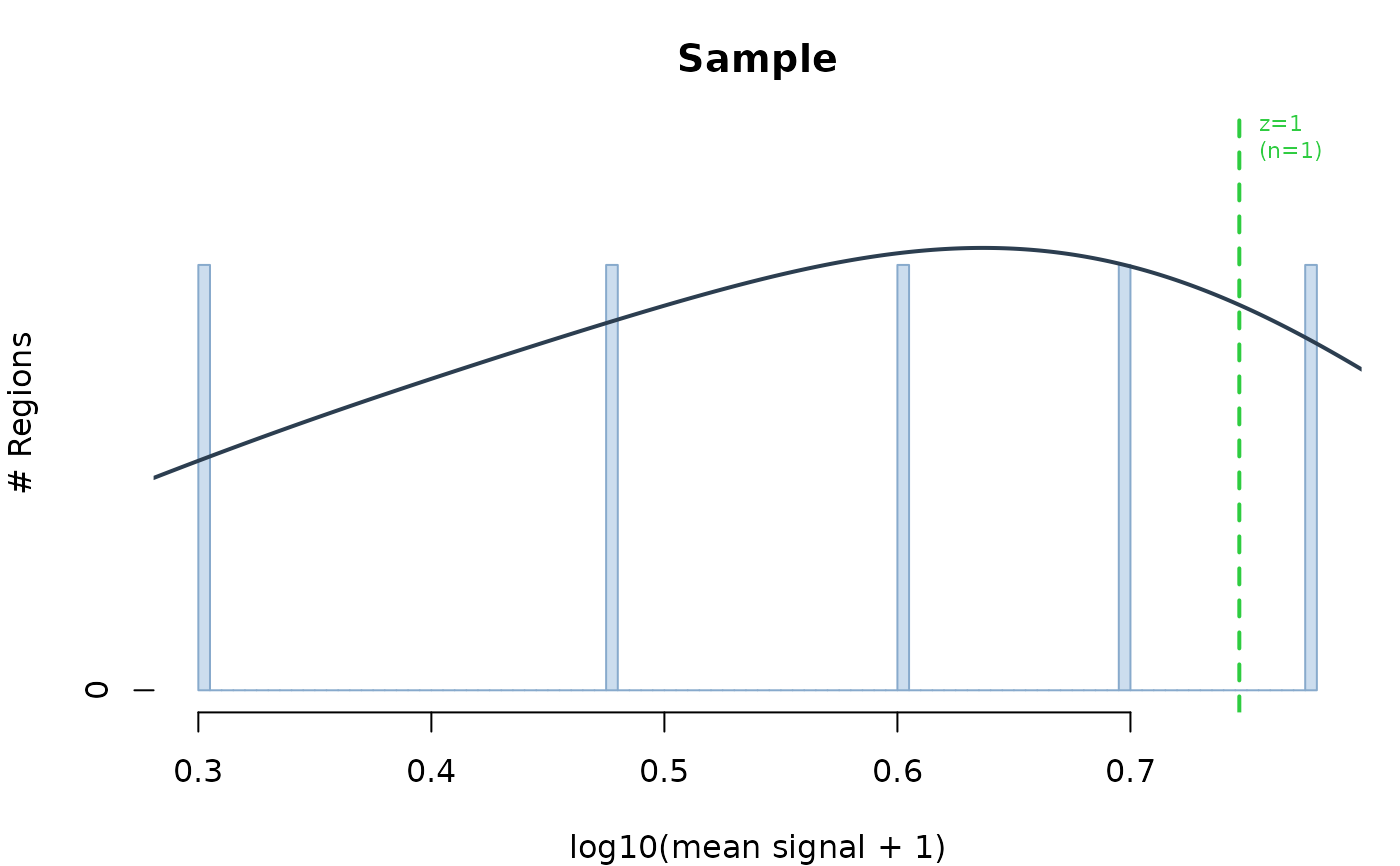
Visualizes the distribution of BigWig signal across genomic regions to help identify the noise floor and select an appropriate z-score or raw signal threshold for calling accessible regions. The distribution is typically bimodal: a large peak at zero/low signal (background noise) and a smaller peak at higher signal (accessible regions).

Usage

plot_signal_histogram(
  bw_paths,
  regions,
  n_bins = 100,
  show_z_lines = base::c(1, 1.5, 2),
  log_scale = TRUE,
  cex_label = 0.7,
  cex_title = 1,
  hist_fill = "#CCDDEE",
  hist_border = "#88AACC",
  density_col = "#2C3E50",
  z_colors = base::c("#2ECC40", "#FF851B", "#E74C3C"),
  suggest_col = "#B10DC9"
)

Arguments

bw_paths: named character vector of BigWig file paths.
regions: GRanges object of regions to examine.
n_bins: integer, number of histogram bins (default: 100).
show_z_lines: numeric vector, z-score thresholds to show as vertical lines (default: c(1.0, 1.5, 2.0)).
log_scale: logical, use log10(signal + 1) for x-axis (default: TRUE).
cex_label: Numeric. Font size for threshold and annotation labels (default 0.7).
cex_title: Numeric. Font size for histogram titles (default 1.0).
hist_fill: character. Histogram bar fill color (default "#CCDDEE").
hist_border: character. Histogram bar border color (default "#88AACC").
density_col: character. Density overlay line color (default "#2C3E50").
z_colors: character vector. Colors for z-score threshold lines (default: green, orange, red).
suggest_col: character. Color for suggested threshold line (default "#B10DC9").

Value

Invisible list of per-sample signal statistics, including mean, sd, quantiles, and suggested thresholds.

Examples

bw_path <- make_example_bigwig()
regions <- GenomicRanges::GRanges(
  "chr1", IRanges::IRanges(
    start = c(1000L, 5000L, 10000L, 20000L, 50000L),
    end   = c(2000L, 6000L, 11000L, 21000L, 51000L)
  )
)
stats <- plot_signal_histogram(c(Sample = bw_path), regions)

file.remove(bw_path)
#> [1] TRUE