Getting Started with epiRomics
Alex M. Mawla & Mark O. Huising
2026-04-20
Source:vignettes/getting-started-with-epiRomics.Rmd
getting-started-with-epiRomics.RmdIntroduction
epiRomics integrates multi-omics data to identify and
visualise enhancer regions from bulk ChIP-seq, histone modification, and
ATAC-seq chromatin accessibility signal, alongside companion RNA-seq.
Its core contribution is a reproducible pipeline that combines
co-occurring histone marks with transcription factor (TF) co-binding to
surface putative enhancers and enhanceosomes, then renders signal,
annotation, and peak tracks together in a single, publication-ready
frame so the biology is immediately inspectable.
The workflow decomposes into four reusable stages that mirror how
epigenomic data is analysed in practice: (1) catalogue every input track
in a single manifest and build an epiRomicsS4 database, (2)
call putative enhancers from any pair of co-occurring histone/ChIP marks
(Creyghton et al. 2010), (3) intersect
those calls against curated enhancer catalogues (FANTOM5 (Andersson et al. 2014), the Islet Regulome
(Miguel-Escalada et al. 2019),
user-supplied BEDs, etc.) to filter for regions supported by an external
reference, and (4) identify enhanceosome regions with dense TF
co-binding and visualise them against the underlying signal. Each stage
is usable on its own: the database alone supports gene-centred track
plots; the filter step accepts any BED-derived reference; the
enhanceosome finder works on either raw or filtered calls.
epiRomics is designed to extend the existing Bioconductor epigenomics
stack rather than replace it. Peak-to-feature annotation reuses
ChIPseeker, genomic-feature overlays compose with
annotatr, BigWig and BED I/O go through
rtracklayer, coordinate algebra and seqinfo harmonisation
use GenomicRanges and GenomeInfoDb, gene
models come from any TxDb.* package, ID mapping from any
org.*.db, and example-data fetching is cached through
BiocFileCache. Static and interactive track viewers such as
Gviz, trackViewer, and Signac
remain the right choice for the scenarios they were built for
(publication-grade track aesthetics, lolliplots, single-cell assays);
epiRomics focuses on the narrower problem of combining
multi-mark bulk data into enhancer and enhanceosome calls and surfacing
them against their own signal for biological interpretation.
Because all gene models come from a user-supplied TxDb.*
and all ID mapping from a user-supplied org.*.db, any
organism available in Bioconductor’s annotation catalogue can be
analysed. This vignette uses human hg38 as a concrete example, but the
same code runs against TxDb.Mmusculus.UCSC.mm10.knownGene +
org.Mm.eg.db,
TxDb.Rnorvegicus.UCSC.rn6.refGene +
org.Rn.eg.db, or any other valid pairing. The
genome string is cross-checked against
GenomeInfoDb::genome(txdb) at build time, so mismatches
fail loudly rather than silently.
This getting-started vignette uses a small toy dataset
(under 1 MB) bundled with the package in inst/extdata/toy/.
The toy subset covers a single 400 kb window on hg38
chr11:1,900,000-2,300,000 centred on the human insulin gene
(INS). A companion vignette, “Full Analysis with
epiRomics”, walks through the complete alpha vs. beta pancreatic
islet analysis using the full 1.3 GB Zenodo archive, available on demand
via epiRomics::cache_data().
Locating the toy data
All toy files live under the package’s installed
inst/extdata/toy/ directory. We resolve the path through
system.file() so the vignette works identically whether it
is rendered from the installed package, during R CMD check,
or from the source tree. The absolute path is machine-specific, so we
only show that the directory resolves and list its basenames.
toy_dir <- system.file("extdata", "toy", package = "epiRomics")
dir.exists(toy_dir)
#> [1] TRUE

list.files(toy_dir)
#> [1] "BED_Annotation"                 "BigWigs"
#> [3] "ChIP"                           "example_epiRomics_BW_sheet.csv"
#> [5] "example_epiRomics_Db_sheet.csv" "Histone"
#> [7] "README.md"                      "toy_database.rds"
The window includes four BigWig signal tracks (alpha/beta ATAC-seq
and RNA-seq), seven histone modification peak sets, five TF ChIP-seq
peak sets, and three enhancer annotation resources. Everything needed to
exercise the full epiRomics pipeline end-to-end is
contained here; nothing is downloaded.
Dataset provenance. The toy bundle is a narrow
subset of a human pancreatic alpha-versus-beta islet dataset that was
curated, reprocessed, and archived on Zenodo (“epiRomics Package
Example Dataset (Curated),” n.d.). The underlying
sequencing data were not generated by the package authors; they were
assembled from published public resources and re-analysed through a
uniform pipeline. The full curation methodology (source accessions,
alignment, peak calling, normalisation) is documented in the package
README. The BigWig tracks here are centred on the hg38 INS
locus (chr11:1,900,000-2,300,000), while the BED peak
catalogues (histone marks, TF ChIP-seq, and curated enhancer references)
are drawn from additional islet loci so the transcription-factor
co-binding analysis below has enough observations for the Fisher
statistic to be informative. The unabridged curated archive (~1.3 GB)
lives on Zenodo and is used by the companion vignette Full Analysis with
epiRomics; it is fetched on demand (and cached locally) via
epiRomics::cache_data(). The reproducibility script that
converts the full archive into this toy subset lives at
inst/scripts/make-toy-data.R.
Installation
epiRomics is installed from Bioconductor:
if (!requireNamespace("BiocManager", quietly = TRUE))
    install.packages("BiocManager")
BiocManager::install("epiRomics")
The organism-specific TxDb.* and org.*.db
packages this vignette uses are listed in Suggests and can
be installed the same way when needed.
Loading the package
This example analyses human hg38 data, so we load
epiRomics together with the hg38 TxDb and the
human org.Hs.eg.db. These annotation packages are declared
in Suggests because epiRomics itself does not
bind to any particular genome: any TxDb.* +
org.*.db pair that Bioconductor ships for an organism
works.
Analysing a different organism. Swap the two annotation packages for the equivalent pair — e.g.
TxDb.Mmusculus.UCSC.mm10.knownGene+org.Mm.eg.dbfor mouse mm10, orTxDb.Rnorvegicus.UCSC.rn6.refGene+org.Rn.eg.dbfor rat rn6. A catalogue ofTxDb.*packages is maintained on the Bioconductor website (https://bioconductor.org/packages/release/BiocViews.html#___TxDb), and a catalogue oforg.*.dbannotations is at (https://bioconductor.org/packages/release/BiocViews.html#___OrgDb). Update thegenome,organism, andtxdb_organismarguments tobuild_database()to match; nothing else in the pipeline changes.
Building the database
The database manifest is a CSV listing every annotation track with
its name, path, genome build,
format, and type. type is one of
histone, methyl, SNP,
chip, or functional. genome is a
free-form string (hg38, mm10,
rn6, …) and is validated against the supplied
TxDb — a mismatch raises an error rather than proceeding
silently.
db_sheet_path <- file.path(toy_dir, "example_epiRomics_Db_sheet.csv")
db_sheet <- read.csv(db_sheet_path)
db_sheet
#>               name
#> 1          h3k27ac
#> 2          h3k4me1
#> 3         h3k27me3
#> 4          h3k9me3
#> 5          h3k4me3
#> 6         h3k36me3
#> 7             h2az
#> 8            foxa2
#> 9             mafb
#> 10          nkx2_2
#> 11          nkx6_1
#> 12            pdx1
#> 13          fantom
#> 14 regulome_active
#> 15  regulome_super
#>                                                       path genome
#> 1                                 Histone/H3k27ac_hg38.bed   hg38
#> 2                                 Histone/H3K4me1_hg38.bed   hg38
#> 3                                Histone/H3K27me3_hg38.bed   hg38
#> 4                                 Histone/H3K9me3_hg38.bed   hg38
#> 5                                 Histone/H3K4me3_hg38.bed   hg38
#> 6                                Histone/H3K36me3_hg38.bed   hg38
#> 7                                    Histone/H2AZ_hg38.bed   hg38
#> 8                                      ChIP/FOXA2_hg38.bed   hg38
#> 9                                       ChIP/MAFB_hg38.bed   hg38
#> 10                                    ChIP/NKX2_2_hg38.bed   hg38
#> 11                                    ChIP/NKX6_1_hg38.bed   hg38
#> 12                                      ChIP/PDX1_hg38.bed   hg38
#> 13              BED_Annotation/Fantom_5.hg38.enhancers.bed   hg38
#> 14 BED_Annotation/Human_Regulome_hg38_Active_Enhancers.bed   hg38
#> 15  BED_Annotation/Human_Regulome_hg38_Super_Enhancers.bed   hg38
#>    format       type
#> 1     bed    histone
#> 2     bed    histone
#> 3     bed    histone
#> 4     bed    histone
#> 5     bed    histone
#> 6     bed    histone
#> 7     bed    histone
#> 8     bed       chip
#> 9     bed       chip
#> 10    bed       chip
#> 11    bed       chip
#> 12    bed       chip
#> 13    bed functional
#> 14    bed functional
#> 15    bed functional
Each row points to a BED file under toy_dir. To extend
the database with your own annotations — for example, an in-house ChIP
peak call set or a curated enhancer list — append additional rows with
the appropriate type and a path relative to the data
directory. build_database() imports every row, attaches
annotation via the supplied TxDb / org.*.db,
and returns an S4 epiRomicsS4 object that all downstream
functions consume. The txdb_organism argument takes a
"package::object" string so the TxDb can be
resolved lazily without forcing an upfront library() call;
live TxDb objects are also accepted.
database <- build_database(
  db_file = db_sheet_path,
  txdb_organism = paste0(
    "TxDb.Hsapiens.UCSC.hg38.knownGene::",
    "TxDb.Hsapiens.UCSC.hg38.knownGene"),
  genome   = "hg38",
  organism = "org.Hs.eg.db",
  data_dir = toy_dir)
build_database() calls
annotatr::build_annotations() which fetches several UCSC
annotation tables (CpG islands, lncRNA transcripts, etc.) the first time
it runs and caches them locally. To keep this vignette
offline-reproducible during R CMD build on the Bioconductor
build farm, we ship a pre-built epiRomicsS4 for the toy
window with the package and load it here instead of rebuilding. The code
above is the canonical invocation every downstream chunk assumes was
run.
#> epiRomicsS4 object
#>   Genome: hg38
#>   Annotations: 8438 ranges
#>   Meta: 15 rows
#>   Organism: org.Hs.eg.db
#>   TxDb: TxDb.Hsapiens.UCSC.hg38.knownGene::TxDb.Hsapiens.UCSC.hg38.knownGene
The returned object holds each imported track together with its genome build and file paths, ready for enhancer discovery.
Quick gene-locus inspection
Before invoking the full pipeline, plot_quick_view()
gives a zero-configuration view of BigWig signal at any gene locus. No
epiRomicsS4 database is required — just a gene symbol, a
named vector of BigWig paths, and a genome string. This is useful for
fast exploration of signal shape at known loci before deciding which
regions to probe with the enhancer pipeline.
We first stage the BigWig track manifest. The paths in the CSV are
relative, so we resolve them against toy_dir; we also
reorder the rows so that beta-cell tracks plot above alpha-cell tracks
in the mirrored view:
track_connection <- read.csv(
  file.path(toy_dir, "example_epiRomics_BW_sheet.csv"))
track_connection$path <- file.path(toy_dir, track_connection$path)

## Reorder: beta tracks first, alpha second
beta_idx  <- grep("Beta",  track_connection$name)
alpha_idx <- grep("Alpha", track_connection$name)
track_connection <- track_connection[c(beta_idx, alpha_idx), ]

## Named vector of BigWig paths and matching colours
bw_paths  <- setNames(track_connection$path, track_connection$name)
bw_colors <- track_connection$color

## Display-friendly view (basenames only); the real data frame
## still holds fully resolved paths for plot_tracks() below.
display_tc <- track_connection
display_tc$path <- basename(display_tc$path)
display_tc
#>                path       name   color type
#> 2  Beta_ATAC.toy.bw  Beta_ATAC #008b00 atac
#> 3   Beta_RNA.toy.bw   Beta_RNA #008b00  rna
#> 1 Alpha_ATAC.toy.bw Alpha_ATAC #e13c64 atac
#> 4  Alpha_RNA.toy.bw  Alpha_RNA #e13c64  rna
The toy BigWigs cover only the INS window on
chr11 (1,900,000-2,300,000), so
plot_quick_view() renders signal for genes inside that
window. The companion Full Analysis vignette demonstrates the
same call against the full-genome BigWigs for multiple beta-cell and
alpha-cell loci (INS, PDX1, MAFA,
GCG, MAFB, UCN3).
plot_quick_view("INS",
  bw_paths = bw_paths,
  colors   = bw_colors,
  mirror   = TRUE,
  genome   = "hg38")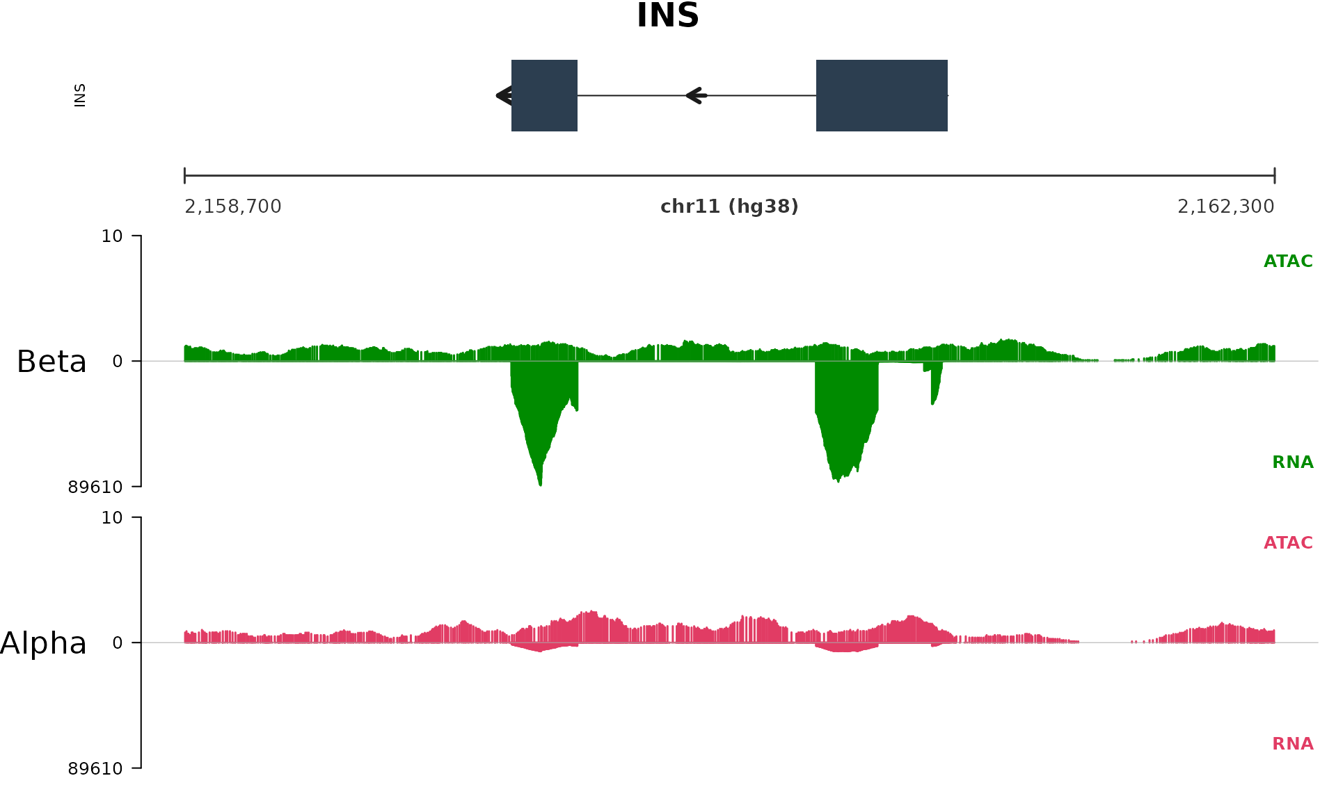
Identifying putative enhancers
Enhancers are canonically identified by the simultaneous presence of
H3K4me1 and H3K27ac (Creyghton et al.
2010), but epiRomics is deliberately general:
find_enhancers_by_comarks() accepts any pair of marks
loaded in the database (columns with type
histone or chip) and returns the regions where
both overlap. That flexibility means the same function can be used to
ask different biological questions — H3K4me1 + H3K27ac for
active enhancers (Creyghton et al.
2010), H3K4me3 + H3K27ac for active promoter-proximal regions
(Heintzman et al. 2009), H3K4me1 +
H3K27me3 for poised enhancers (Rada-Iglesias et al. 2011), H2A.Z + H3K27ac for
primed regions (Ernst and Kellis 2012; Kundaje et
al. 2015), etc. The choice of marks encodes the hypothesis; the
function signature does not change. ChromHMM-style combinatorial states
summarising these are revisited in the Chromatin state
classification section below.
epiRomicsS4 objects expose their five slots through
public getter functions: annotations(),
meta(), txdb(), organism(), and
genome(). Users should prefer these accessors over reaching
into slots directly with @ or slot() — they
are the stable public API for reading and (via <-
assignment) writing slot contents.
putative_enhancers <- find_enhancers_by_comarks(
  database,
  histone_mark_1 = "h3k4me1",
  histone_mark_2 = "h3k27ac")

head(as.data.frame(annotations(putative_enhancers)), 5)
#>   seqnames   start     end width strand
#> 1    chr11 2076702 2077260   559      *
#> 2    chr11 2092612 2093857  1246      *
#> 3    chr11 2096933 2096999    67      *
#> 4    chr11 2097154 2097349   196      *
#> 5    chr11 2097525 2097677   153      *
The resulting epiRomicsS4 object carries the co-marked
regions in its annotations slot as a GRanges-like data
frame — the genomic coordinates and feature metadata for each putative
enhancer. We inspect the slot via the annotations() getter
throughout this vignette; the key columns are
seqnames/start/end (genomic
coordinates), annotation (genic context from
ChIPseeker), and distanceToTSS (signed
distance to the nearest transcription start site).
Cross-referencing against curated enhancer databases
Putative enhancers gain biological weight when they overlap regions
from a trusted reference. filter_enhancers() intersects the
putative calls against any row whose type is
functional in the database manifest. The reference to use
is selected with the type argument, which follows the
convention "{genome}_custom_{name}" where
name matches the name column of the
functional row. The toy dataset ships with three functional references
already loaded:
type argument |
Reference |
|---|---|
hg38_custom_fantom |
FANTOM5 permissive enhancer atlas |
hg38_custom_regulome_active |
Human Islet Regulome — active enhancers |
hg38_custom_regulome_super |
Human Islet Regulome — super-enhancers |
To add additional references — an in-house enhancer catalogue, a
differentially-accessible chromatin region list, ChromHMM state calls,
disease-variant BEDs, or any other BED-valued resource — append a new
row to the manifest CSV with type = "functional" and the
corresponding name. After rebuilding the database, the new
row is accessible via
filter_enhancers(..., type = "hg38_custom_<name>").
No code changes are required.
fantom_enhancers <- filter_enhancers(
  putative_enhancers,
  database,
  type = "hg38_custom_fantom")

head(as.data.frame(annotations(fantom_enhancers)), 5)
#>   seqnames   start     end width strand
#> 1    chr11 2202659 2203222   564      *
The Human Islet Regulome (Miguel-Escalada et al. 2019) supplies an orthogonal, tissue-specific catalogue. We cross-reference the same putative calls against its active enhancer set, and separately against its super-enhancer set:
regulome_enhancers <- filter_enhancers(
  putative_enhancers,
  database,
  type = "hg38_custom_regulome_active")

head(as.data.frame(annotations(regulome_enhancers)), 5)
#>   seqnames   start     end width strand
#> 1    chr11 2176013 2176162   150      *
#> 2    chr11 2201955 2202411   457      *
#> 3    chr11 2202659 2203222   564      *
#> 4    chr11 2208420 2208667   248      *
#> 5    chr11 2208885 2209771   887      *
regulome_super_enhancers <- filter_enhancers(
  putative_enhancers,
  database,
  type = "hg38_custom_regulome_super")

head(as.data.frame(annotations(regulome_super_enhancers)), 5)
#>   seqnames   start     end width strand
#> 1    chr11 2176013 2176162   150      *
#> 2    chr11 2193633 2194043   411      *
#> 3    chr11 2201955 2202411   457      *
#> 4    chr11 2202659 2203222   564      *
#> 5    chr11 2208420 2208667   248      *
Each filter narrows the putative set to the subset supported by the chosen reference. Downstream steps can operate on either filtered object (or all three, to compare reference-agreement).
Identifying enhanceosome regions
Enhanceosomes are enhancer regions with high TF co-binding.
find_enhanceosomes() intersects putative (or filtered)
enhancers with every ChIP-seq track in the database and sorts the result
by co-binding count, so the densest regulatory regions sort to the
top.
Here we feed the broader putative_enhancers set (rather
than a reference-filtered subset) into find_enhanceosomes()
so the TF co-binding demo has statistical power across all four islet
loci represented in the toy BEDs (INS, GCG, PDX1, MAFB). Filtering
against FANTOM5 or the Islet Regulome first would collapse the call set
to the narrow BigWig window and leave the Fisher tests underpowered; in
practice users chain either the filtered or the unfiltered set into
find_enhanceosomes() depending on their hypothesis.
enhanceosomes <- find_enhanceosomes(
  putative_enhancers,
  database)
#> >> preparing features information...      2026-04-20 23:35:02
#> >> Using Genome: hg38 ...
#> >> identifying nearest features...        2026-04-20 23:35:03
#> >> calculating distance from peak to TSS...   2026-04-20 23:35:03
#> >> assigning genomic annotation...        2026-04-20 23:35:03
#> >> Using Genome: hg38 ...
#> >> Using Genome: hg38 ...
#> >> adding gene annotation...          2026-04-20 23:35:42
#> 'select()' returned 1:1 mapping between keys and columns
#> >> assigning chromosome lengths           2026-04-20 23:35:42
#> >> done...                    2026-04-20 23:35:42

head(as.data.frame(annotations(enhanceosomes)), 5)
#>   seqnames   start     end width strand foxa2 mafb nkx2_2 nkx6_1 pdx1
#> 1    chr11 2210208 2211181   974      *     1    1      1      1    1
#> 2    chr11 2176013 2176162   150      *     0    1      1      0    1
#> 3    chr11 2211584 2211983   400      *     1    0      1      0    1
#> 4    chr11 2076702 2077260   559      *     1    0      0      0    0
#> 5    chr11 2099922 2100126   205      *     0    0      1      0    0
#>   ChIP_Hits
#> 1         5
#> 2         3
#> 3         3
#> 4         1
#> 5         1
#>                                                    annotation geneChr
#> 1                                           Distal Intergenic      11
#> 2                                            Promoter (2-3kb)      11
#> 3                                           Distal Intergenic      11
#> 4 Intron (ENST00000796724.1/ENST00000796724.1, intron 2 of 3)      11
#> 5                                           Distal Intergenic      11
#>   geneStart geneEnd geneLength geneStrand    geneId      transcriptId
#> 1   2173063 2173138         76          1 100616126 ENST00000584128.1
#> 2   2173063 2173138         76          1 100616126 ENST00000584128.1
#> 3   2173063 2173138         76          1 100616126 ENST00000584128.1
#> 4   2134134 2134209         76          2    619552 ENST00000385070.3
#> 5   2134134 2134209         76          2    619552 ENST00000385070.3
#>   distanceToTSS         ENSEMBL  SYMBOL      GENENAME
#> 1         37145 ENSG00000265258 MIR4686 microRNA 4686
#> 2          2950 ENSG00000265258 MIR4686 microRNA 4686
#> 3         38521 ENSG00000265258 MIR4686 microRNA 4686
#> 4         56949 ENSG00000207805  MIR483  microRNA 483
#> 5         34083 ENSG00000207805  MIR483  microRNA 483

length(annotations(enhanceosomes))
#> [1] 20
The first rows list the most densely co-bound regions, ranked by the number of TFs binding each; the final value reports the total number of enhanceosome calls recovered across the toy BED window.
TF co-binding statistics
analyze_tf_cobinding() runs a Fisher’s exact test on
each pair of TFs represented in the enhanceosome set and reports odds
ratios and point-wise mutual information (PMI), so statistically
enriched partnerships can be flagged directly.
tf_stats <- analyze_tf_cobinding(enhanceosomes, database)
tf_stats$pairwise
#>       tf1    tf2 n_both n_tf1_only n_tf2_only n_neither odds_ratio
#> 1   foxa2 nkx6_1      1          2          0        17        Inf
#> 2    mafb nkx2_2      2          0          7        11        Inf
#> 3    mafb nkx6_1      1          1          0        18        Inf
#> 4    mafb   pdx1      2          0          1        17        Inf
#> 5  nkx2_2 nkx6_1      1          8          0        11        Inf
#> 6  nkx2_2   pdx1      3          6          0        11        Inf
#> 7  nkx6_1   pdx1      1          0          2        17        Inf
#> 8   foxa2   pdx1      2          1          1        16    21.6987
#> 9   foxa2   mafb      1          2          1        16     6.7328
#> 10  foxa2 nkx2_2      2          1          7        10     2.7097
#>      pvalue    pmi      fdr significant
#> 1  0.150000 2.7370 0.250000       FALSE
#> 2  0.189474 1.1520 0.270677       FALSE
#> 3  0.100000 3.3219 0.250000       FALSE
#> 4  0.015789 2.7370 0.157895       FALSE
#> 5  0.450000 1.1520 0.500000       FALSE
#> 6  0.073684 1.1520 0.245614       FALSE
#> 7  0.150000 2.7370 0.250000       FALSE
#> 8  0.045614 2.1520 0.228070       FALSE
#> 9  0.284211 1.7370 0.355263       FALSE
#> 10 0.565789 0.5670 0.565789       FALSE
Each row reports one TF pair with: tf1/tf2
(factor names),
n_both/n_tf1_only/n_tf2_only/n_neither
(2x2 contingency counts of enhanceosomes), odds_ratio
(Fisher’s test effect size; >1 indicates enrichment),
pvalue and fdr (Benjamini-Hochberg adjusted),
pmi (pointwise mutual information), and
significant (TRUE when FDR below threshold and
n_both above the min_regions floor).
Statistical power here is bounded by the size of the toy dataset; on the
full dataset the same call surfaces canonical islet TF partnerships such
as FOXA2 + PDX1 with substantially stronger significance. The “Full
Analysis with epiRomics” vignette works through the full-scale
result.
Visualising an enhanceosome with signal tracks
plot_tracks() renders the selected enhanceosome region
with its supporting ChIP-seq, histone, annotation, and BigWig signal
tracks stacked for direct visual comparison. By default, paired ATAC and
RNA signals for matched cell types are plotted in a
mirrored layout (mirror = TRUE), with one
cell type above the axis and the other below — this makes
cell-type-specific differences read at a glance. Setting
mirror = FALSE falls back to a single-direction layout with
each track stacked in its own panel.
The toy BigWigs cover only the INS window on
chr11, while the enhanceosome set spans all four toy loci.
To get a track plot with live BigWig signal we pick the first
enhanceosome that falls inside the BigWig window; outside that window
the signal panels would be empty.
enh_df <- as.data.frame(annotations(enhanceosomes))
in_window <- which(
  enh_df$seqnames == "chr11" &
    enh_df$start >= 1900000 &
    enh_df$end   <= 2300000)
length(in_window)
#> [1] 20
selected_index <- in_window[1]
selected_index
#> [1] 1
enh_df[selected_index, c("seqnames", "start", "end")]
#>   seqnames   start     end
#> 1    chr11 2210208 2211181
plot_tracks(
  enhanceosomes,
  index = selected_index,
  database = database,
  track_connection = track_connection)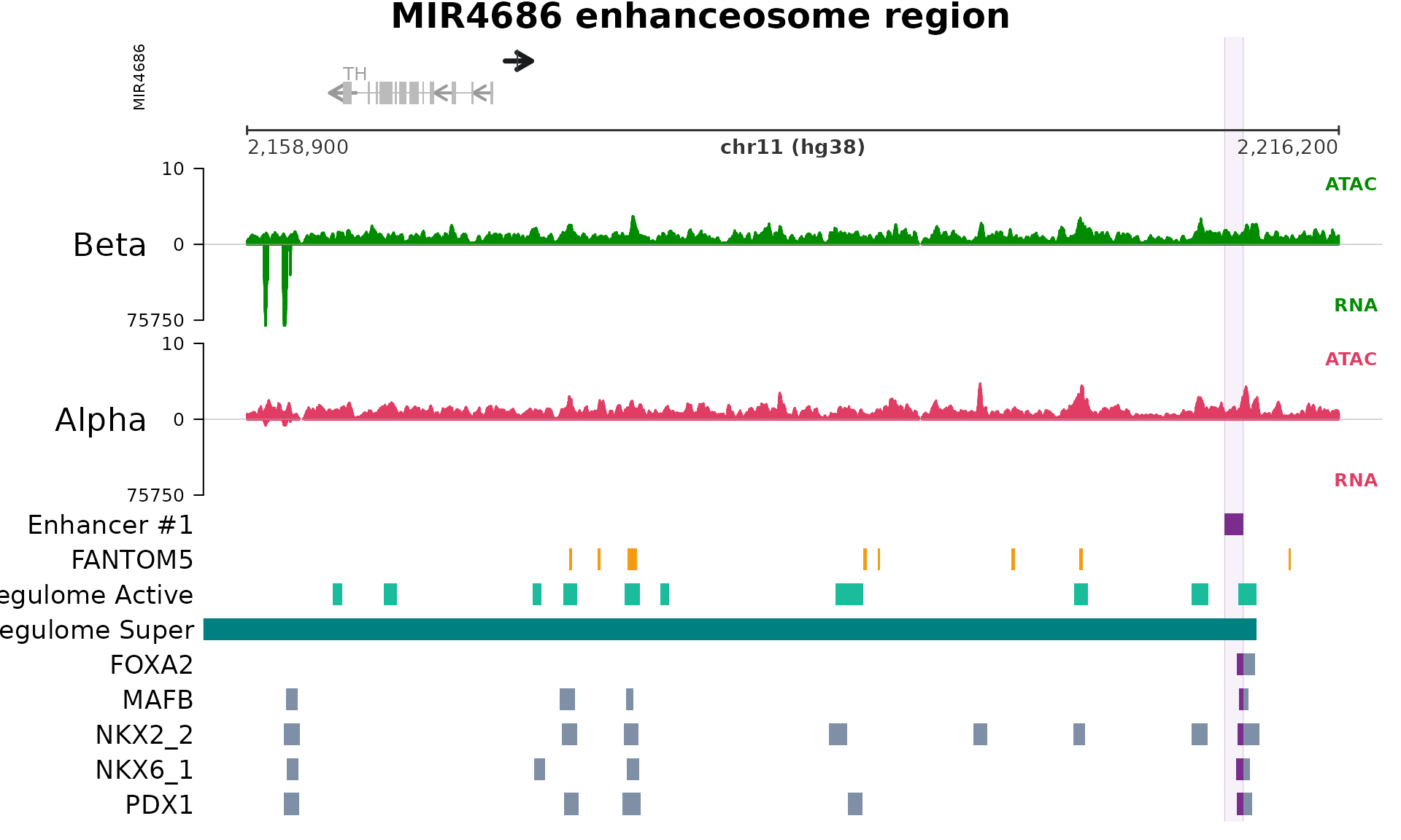
Reading the figure (top → bottom): the gene model panel anchors the locus and shows nearby transcripts, with the focal gene highlighted; the coordinate bar beneath it marks genomic position; the middle block holds the mirrored signal tracks (alpha-cell tracks above the axis, beta-cell tracks below); the highlighted vertical span marks the enhanceosome interval; and the histone-mark and TF peak annotation panels at the bottom indicate which of the database’s tracks contributed to the call.
Gene-centred visualisation
plot_gene_tracks() takes a gene symbol and renders every
database track alongside the BigWig signal in a gene-centred frame.
Because the toy window was built around INS, this call
reproduces the canonical islet insulin locus view at toy-level bundle
size.
plot_gene_tracks("INS", database, track_connection)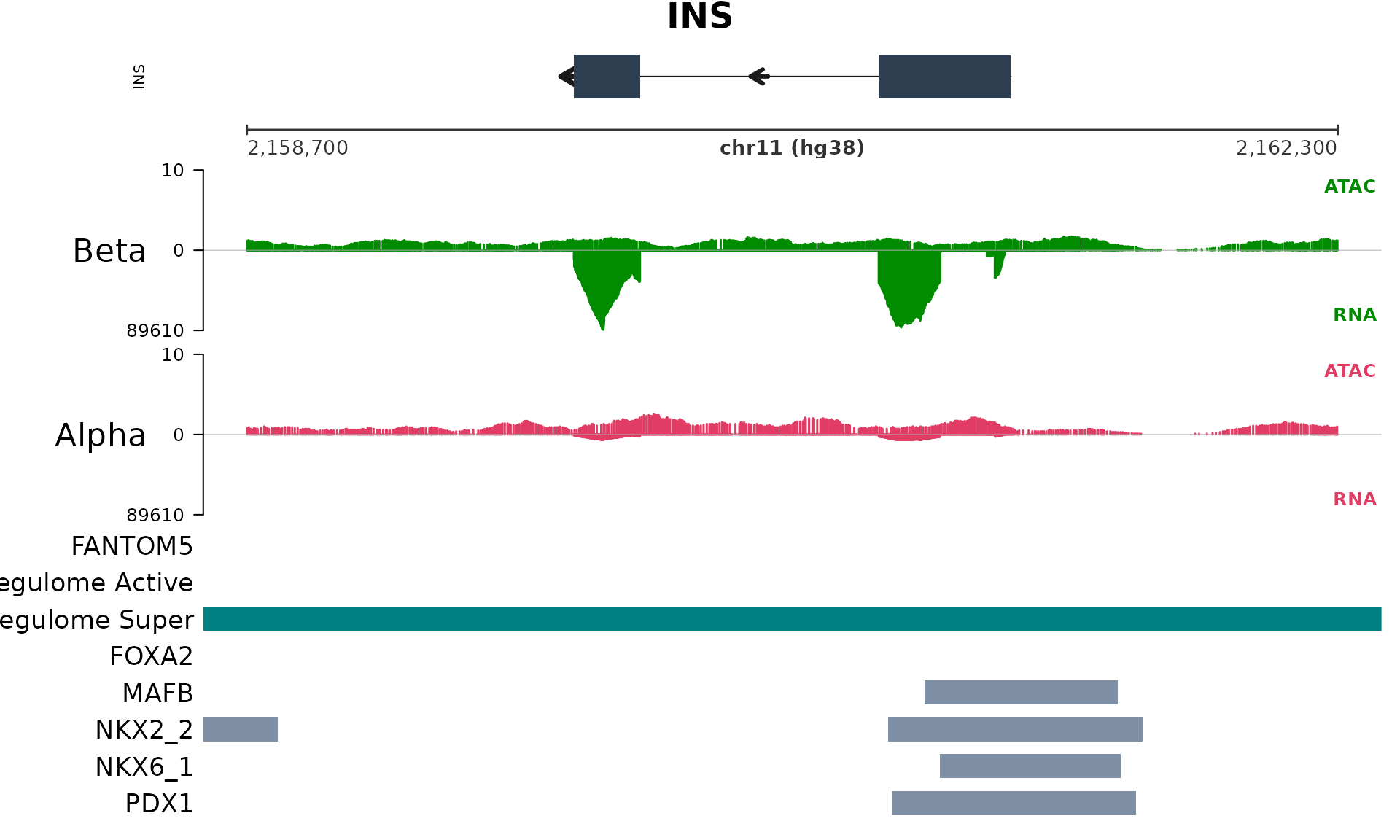
Chromatin state classification
classify_chromatin_states() labels genomic regions using
their combinations of histone marks, producing six ChromHMM-style states
(Ernst and Kellis 2012; Kundaje et al.
2015). TSS proximity is incorporated to refine the
classification. The six labels are:
| State | Defining marks | Interpretation |
|---|---|---|
active |
H3K4me1 + H3K27ac | Active enhancer or active regulatory element (Creyghton et al. 2010) |
bivalent |
H3K4me3 + H3K27me3 | Poised developmental promoter held in a balance of activating and repressive marks |
poised |
H3K4me1 + H3K27me3 | Poised enhancer — primed but held repressed |
primed |
H3K4me1 only | Primed enhancer — accessible but not yet active |
repressed |
H3K27me3 (or H3K9me3) without activating marks | Polycomb-repressed or heterochromatic region |
unmarked |
None of the above | No informative histone signal in the input set |
chromatin_states <- classify_chromatin_states(database)
table(chromatin_states$chromatin_state)
#>
#>    active  bivalent    poised    primed repressed  unmarked
#>        16         2         1        16        23        18
table(chromatin_states$genomic_context)
#>
#>  gene_body intergenic   promoter
#>          6         63          7
The tables above summarise how many regions fall into each state and each genomic context (promoter, intron, distal) within the toy window.
Chromatin-state calls can be overlaid directly on a gene-centred
track plot by passing the chromatin_states data frame
together with show_chromatin = TRUE:
plot_gene_tracks("INS",
  database,
  track_connection,
  chromatin_states = chromatin_states,
  show_chromatin = TRUE,
  show_enhancer_highlight = TRUE)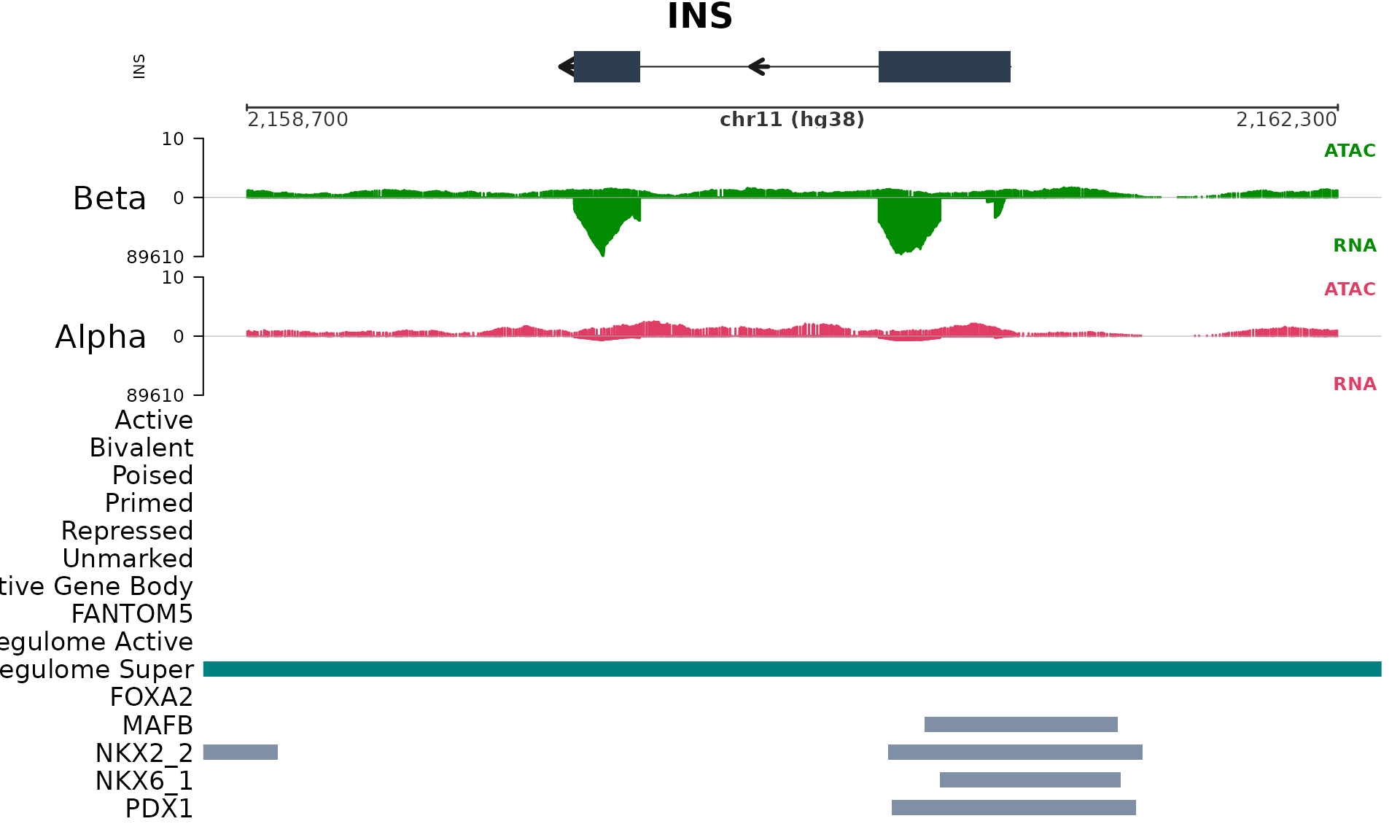
The overlay highlights where active, bivalent, poised, primed, repressed, or unmarked states land relative to gene bodies and signal — a useful sanity check before moving from enhanceosome calls to downstream biological interpretation.
Moving on to the full dataset
This vignette exercises the core enhancer-discovery and visualisation pipeline on a 400 kb toy window. For the complete alpha-vs-beta pancreatic islet analysis — including differential chromatin accessibility integration and the full set of enhanceosome calls — see the companion vignette “Full Analysis with epiRomics”. That walkthrough uses the full 1.3 GB Zenodo archive, which is fetched once with:
epiRomics::cache_data()The archive is stored in a BiocFileCache, so subsequent
runs reuse the download.
Interactive showcases
Two companion Shiny applications render published enhanceosome
browsers built with epiRomics:
- Shiny epiRomics Mouse Islet Enhanceosome Browser — mouse pancreatic alpha, beta, and delta cell results from (Mawla, Meulen, and Huising 2023).
- Shiny epiRomics Human Islet Enhanceosome Browser — human alpha and beta cell results used as the example dataset for this package (Mawla and Huising 2021).
Citation
If you use epiRomics in published research, please cite
both (Mawla, Meulen, and Huising 2023) and
(Mawla and Huising 2021) (full entries
appear in the References section below). A ready-to-paste BibTeX block
is also available via:
citation("epiRomics")Session information
sessionInfo()
#> R version 4.5.3 (2026-03-11)
#> Platform: x86_64-pc-linux-gnu
#> Running under: Ubuntu 24.04.4 LTS
#>
#> Matrix products: default
#> BLAS:   /usr/lib/x86_64-linux-gnu/openblas-pthread/libblas.so.3
#> LAPACK: /usr/lib/x86_64-linux-gnu/openblas-pthread/libopenblasp-r0.3.26.so;  LAPACK version 3.12.0
#>
#> locale:
#>  [1] LC_CTYPE=C.UTF-8       LC_NUMERIC=C
#>  [3] LC_TIME=C.UTF-8        LC_COLLATE=C.UTF-8
#>  [5] LC_MONETARY=C.UTF-8    LC_MESSAGES=C.UTF-8
#>  [7] LC_PAPER=C.UTF-8       LC_NAME=C
#>  [9] LC_ADDRESS=C           LC_TELEPHONE=C
#> [11] LC_MEASUREMENT=C.UTF-8 LC_IDENTIFICATION=C
#>
#> time zone: UTC
#> tzcode source: system (glibc)
#>
#> attached base packages:
#> [1] stats4    stats     graphics  grDevices utils     datasets
#> [7] methods   base
#>
#> other attached packages:
#>  [1] org.Hs.eg.db_3.22.0
#>  [2] TxDb.Hsapiens.UCSC.hg38.knownGene_3.22.0
#>  [3] GenomicFeatures_1.62.0
#>  [4] AnnotationDbi_1.72.0
#>  [5] Biobase_2.70.0
#>  [6] GenomicRanges_1.62.1
#>  [7] Seqinfo_1.0.0
#>  [8] IRanges_2.44.0
#>  [9] S4Vectors_0.48.1
#> [10] BiocGenerics_0.56.0
#> [11] generics_0.1.4
#> [12] epiRomics_0.99.5
#>
#> loaded via a namespace (and not attached):
#>   [1] splines_4.5.3
#>   [2] BiocIO_1.20.0
#>   [3] bitops_1.0-9
#>   [4] ggplotify_0.1.3
#>   [5] filelock_1.0.3
#>   [6] tibble_3.3.1
#>   [7] R.oo_1.27.1
#>   [8] polyclip_1.10-7
#>   [9] XML_3.99-0.23
#>  [10] lifecycle_1.0.5
#>  [11] httr2_1.2.2
#>  [12] lattice_0.22-9
#>  [13] MASS_7.3-65
#>  [14] magrittr_2.0.5
#>  [15] sass_0.4.10
#>  [16] rmarkdown_2.31
#>  [17] jquerylib_0.1.4
#>  [18] yaml_2.3.12
#>  [19] plotrix_3.8-14
#>  [20] ggtangle_0.1.1
#>  [21] cowplot_1.2.0
#>  [22] DBI_1.3.0
#>  [23] RColorBrewer_1.1-3
#>  [24] abind_1.4-8
#>  [25] purrr_1.2.2
#>  [26] R.utils_2.13.0
#>  [27] RCurl_1.98-1.18
#>  [28] yulab.utils_0.2.4
#>  [29] tweenr_2.0.3
#>  [30] rappdirs_0.3.4
#>  [31] gdtools_0.5.0
#>  [32] enrichplot_1.30.5
#>  [33] ggrepel_0.9.8
#>  [34] tidytree_0.4.7
#>  [35] pkgdown_2.2.0
#>  [36] ChIPseeker_1.46.1
#>  [37] codetools_0.2-20
#>  [38] DelayedArray_0.36.1
#>  [39] DOSE_4.4.0
#>  [40] ggforce_0.5.0
#>  [41] tidyselect_1.2.1
#>  [42] aplot_0.2.9
#>  [43] UCSC.utils_1.6.1
#>  [44] farver_2.1.2
#>  [45] matrixStats_1.5.0
#>  [46] BiocFileCache_3.0.0
#>  [47] GenomicAlignments_1.46.0
#>  [48] jsonlite_2.0.0
#>  [49] annotatr_1.36.0
#>  [50] systemfonts_1.3.2
#>  [51] tools_4.5.3
#>  [52] ggnewscale_0.5.2
#>  [53] treeio_1.34.0
#>  [54] TxDb.Hsapiens.UCSC.hg19.knownGene_3.22.1
#>  [55] ragg_1.5.2
#>  [56] Rcpp_1.1.1-1
#>  [57] glue_1.8.1
#>  [58] SparseArray_1.10.10
#>  [59] xfun_0.57
#>  [60] qvalue_2.42.0
#>  [61] MatrixGenerics_1.22.0
#>  [62] GenomeInfoDb_1.46.2
#>  [63] dplyr_1.2.1
#>  [64] withr_3.0.2
#>  [65] BiocManager_1.30.27
#>  [66] fastmap_1.2.0
#>  [67] boot_1.3-32
#>  [68] caTools_1.18.3
#>  [69] digest_0.6.39
#>  [70] R6_2.6.1
#>  [71] gridGraphics_0.5-1
#>  [72] textshaping_1.0.5
#>  [73] GO.db_3.22.0
#>  [74] gtools_3.9.5
#>  [75] RSQLite_2.4.6
#>  [76] cigarillo_1.0.0
#>  [77] R.methodsS3_1.8.2
#>  [78] tidyr_1.3.2
#>  [79] fontLiberation_0.1.0
#>  [80] data.table_1.18.2.1
#>  [81] rtracklayer_1.70.1
#>  [82] httr_1.4.8
#>  [83] htmlwidgets_1.6.4
#>  [84] S4Arrays_1.10.1
#>  [85] scatterpie_0.2.6
#>  [86] regioneR_1.42.0
#>  [87] pkgconfig_2.0.3
#>  [88] gtable_0.3.6
#>  [89] blob_1.3.0
#>  [90] S7_0.2.1-1
#>  [91] XVector_0.50.0
#>  [92] htmltools_0.5.9
#>  [93] fontBitstreamVera_0.1.1
#>  [94] fgsea_1.36.2
#>  [95] scales_1.4.0
#>  [96] png_0.1-9
#>  [97] ggfun_0.2.0
#>  [98] knitr_1.51
#>  [99] tzdb_0.5.0
#> [100] reshape2_1.4.5
#> [101] rjson_0.2.23
#> [102] nlme_3.1-168
#> [103] curl_7.0.0
#> [104] cachem_1.1.0
#> [105] stringr_1.6.0
#> [106] BiocVersion_3.22.0
#> [107] KernSmooth_2.23-26
#> [108] parallel_4.5.3
#> [109] restfulr_0.0.16
#> [110] desc_1.4.3
#> [111] pillar_1.11.1
#> [112] grid_4.5.3
#> [113] vctrs_0.7.3
#> [114] gplots_3.3.0
#> [115] tidydr_0.0.6
#> [116] dbplyr_2.5.2
#> [117] cluster_2.1.8.2
#> [118] evaluate_1.0.5
#> [119] readr_2.2.0
#> [120] cli_3.6.6
#> [121] compiler_4.5.3
#> [122] Rsamtools_2.26.0
#> [123] rlang_1.2.0
#> [124] crayon_1.5.3
#> [125] plyr_1.8.9
#> [126] fs_2.1.0
#> [127] ggiraph_0.9.6
#> [128] stringi_1.8.7
#> [129] BiocParallel_1.44.0
#> [130] Biostrings_2.78.0
#> [131] lazyeval_0.2.3
#> [132] GOSemSim_2.36.0
#> [133] fontquiver_0.2.1
#> [134] Matrix_1.7-4
#> [135] BSgenome_1.78.0
#> [136] hms_1.1.4
#> [137] patchwork_1.3.2
#> [138] bit64_4.6.0-1
#> [139] ggplot2_4.0.2
#> [140] KEGGREST_1.50.0
#> [141] SummarizedExperiment_1.40.0
#> [142] AnnotationHub_4.0.0
#> [143] igraph_2.2.3
#> [144] memoise_2.0.1
#> [145] bslib_0.10.0
#> [146] ggtree_4.0.5
#> [147] fastmatch_1.1-8
#> [148] bit_4.6.0
#> [149] ape_5.8-1